Mathematical Details

Installation | Core concepts | Mechanisms | Patterns | Mathematical details | Benchmarking workflow | API reference

This page describes how TSGap turns a complete time-series array into (X_missing, mask). The goal is to make the probability calculations and mask construction explicit enough for reproducible benchmarking.

TSGap separates missingness into two steps:

1. A mechanism decides why entries are selected for missingness.

2. A pattern rearranges those selected entries in time.

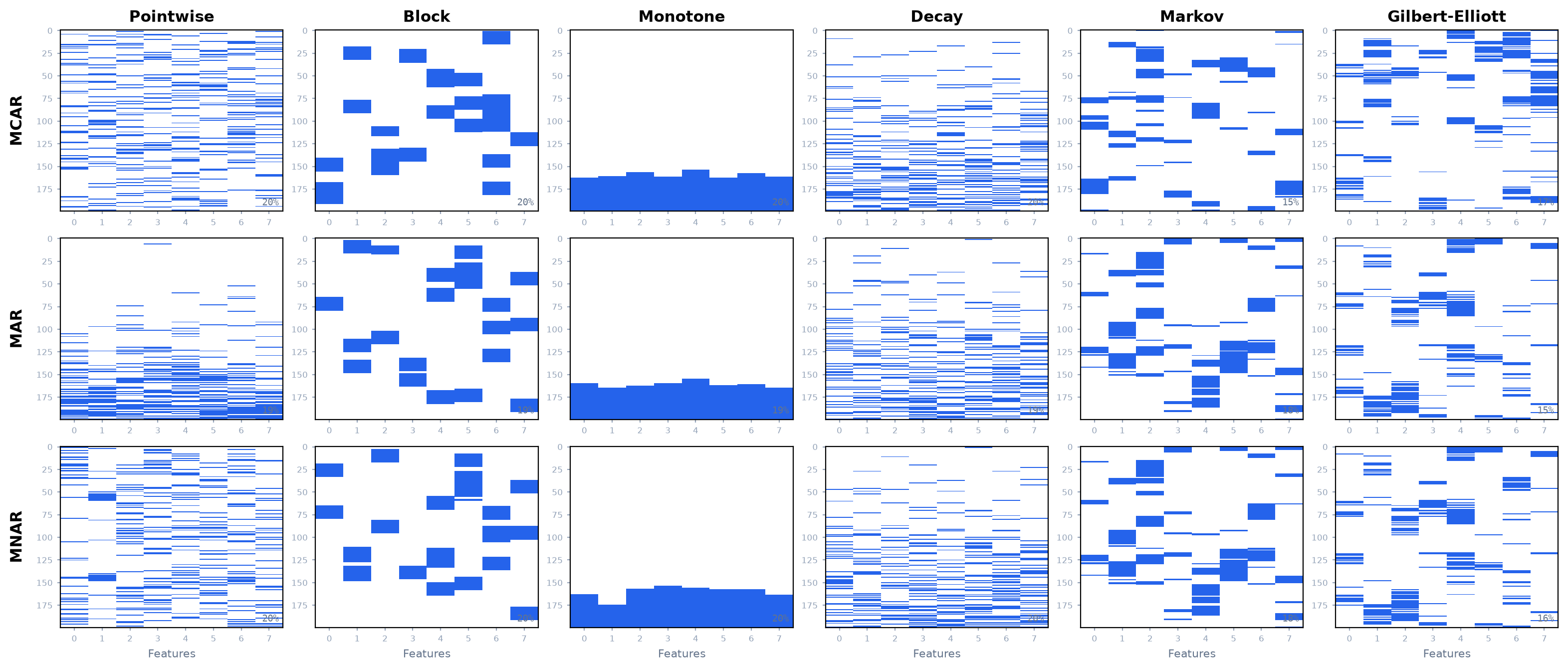
The returned mask uses:

mask == True  -> observed
mask == False -> missing

Intuition: A Plain-Language Walkthrough

If you are new to the math, start here. This section explains every idea and symbol in everyday language before the formal definitions below.

The big picture

Imagine a spreadsheet of sensor readings — rows are moments in time, columns are different measurements (heart rate, temperature, and so on). TSGap’s job is to poke “holes” in this spreadsheet on purpose: deleting some values so you can later test whether an imputation program can guess them back correctly.

Real data does not lose values randomly, so TSGap pokes holes in realistic ways. That is what all the math is for. It happens in two steps: first decide which values disappear (the mechanism), then decide how the gaps are shaped over time (the pattern).

The basic ingredients

• X (your data). The spreadsheet. Shape (T, D) is one subject: T rows (timesteps) and D columns (features). Shape (N, T, D) is N subjects stacked together. Two shapes exist because sometimes you study one patient over time, sometimes many patients at once.

• r (the missing rate). The fraction of values to delete. r = 0.15 means “delete 15%.” It is forced between 0 and 1 — you cannot delete 150% of your data.

• E (the eligible set). The cells we are allowed to delete. We exclude cells that are already blank (you cannot delete a blank) and columns you asked to leave alone. We need this so we only measure holes we made, not ones that were already there.

• mask (the answer key). A true/false grid the same size as the data. True = still here, False = we deleted it. It tells you exactly which cells you poked out so you can score an imputation method fairly.

Step 1: Which values to delete (the mechanism)

There are three styles, each a different reason data goes missing.

MCAR — totally random. Every eligible cell has an equal chance, like drawing names from a hat. We compute how many to delete, m = round(r * |E|), then draw exactly that many. Here |E| is the number of eligible cells. This is exact.

MAR — missing because of another measurement. Example: a heart-rate sensor fails more during hard exercise. The heart rate goes missing, but the cause is activity level (a column we can still see).

• y_t (driver signal). We combine one or more “driver” columns into a single number per timestep. With multiple drivers we use weights w_k (say activity 80%, temperature 20%). The normalized weights w̃_k are just the weights divided by their total so they add up to 1 — this keeps the scale sensible no matter what numbers you type.

• s_t (normalized signal). We rescale y to have average 0 and spread 1 using s = (y - mean) / std. The mean centers it; the std (standard deviation, a measure of spread) puts everything on a common scale. Without this, a heart rate (~70) and a temperature (~37) would not be comparable.

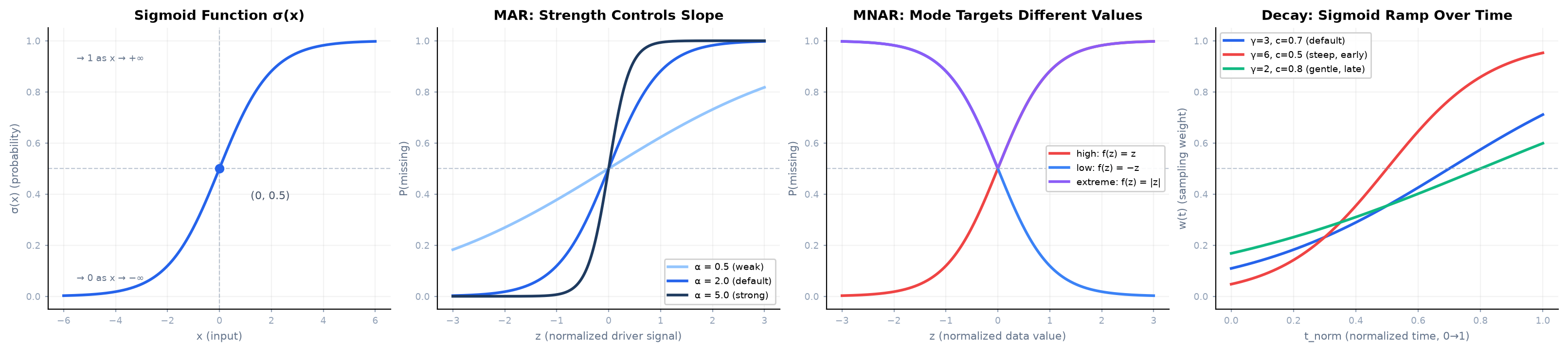
• The sigmoid σ. An S-shaped function that squishes any number into a probability between 0 and 1. Big positive input → near 1 (almost surely delete); big negative → near 0 (almost surely keep); 0 → 0.5 (coin flip).

• α (strength). How steep the S is — how strongly the driver matters. Big α = the driver dramatically changes the odds; small α = it barely matters.

• β (offset). A knob that slides the S left or right to control the overall deletion rate. You do not set it by hand; TSGap finds it automatically (see calibration below).

• base_rate (floor). A minimum deletion chance so even “safe” values are not fully protected. It is capped at half the target rate so it never contradicts a low r.

MNAR — missing because of its own value. Example: a thermometer maxes out and cannot record extreme heat, so the reading vanishes because it was too high. We z-score the value itself (z = (X - mean) / std) and pick a score: z targets high values, -z targets low values, |z| targets both extremes. Then the same sigmoid turns the score into a probability.

Calibration: finding β automatically

You want exactly 20% missing, but the sigmoid gives whatever it gives. TSGap plays “guess the number” (binary search) on β: guess a value, check the resulting rate, nudge up if too low or down if too high, and keep halving the range until it is close. This works because raising β always raises the rate, so the search always closes in.

Sampling: flipping the coins

Every eligible cell now has a probability p. We draw a random number u between 0 and 1 and delete the cell if u ≤ p. A bigger p means a bigger “delete zone,” so it is more likely to go. Because this is coin-flipping, MAR and MNAR hit the target rate approximately; MCAR is exact because it draws a fixed count instead.

Step 2: How the gaps are shaped in time (the pattern)

Step 1 chose which cells and how many. Step 2 rearranges them into realistic shapes while keeping the same total count.

• Pointwise. Do nothing; holes stay scattered like sprinkles.

• Block. Group holes into solid chunks (a sensor offline for 10 minutes). block_density sets how many holes go into chunks versus staying scattered; block_len sets chunk length in steps; block_frac sets it as a fraction of total time (so it scales to long recordings), and a range makes chunk lengths vary.

• Monotone. Once it breaks, it stays broken (a patient drops out for good). The dropout time τ = T - (missing count for that series) is the moment a series goes dark forever. Series the mechanism hit harder go dark earlier.

• Decay. Holes grow more common over time (a dying battery). A time weight w(t) = σ(decay_rate * (t_norm - decay_center)) makes later steps more likely to be chosen. decay_center is where failure crosses 50% (0.7 = last 30%); decay_rate controls how sharp the drop-off is.

• Markov. Flickering on and off (a loose connection). persist is the chance a broken sensor stays broken next step (high = long outages). The onset probability (chance a working sensor breaks) is solved automatically so the long-run average matches the target rate.

• Gilbert-Elliott. A more realistic version of flickering (bursty packet loss). The sensor alternates between “good” and “bad” periods, but a bad period only loses data most of the time (bad_loss), and a good period can still drop the occasional value (good_loss). This makes bursts look ragged rather than perfectly on/off.

Step 3: Finishing up

Cells marked False become NaN in the output, pre-existing blanks stay blank, and using the same seed always reproduces the exact same holes. The formal definitions of everything above follow in the rest of this page.

Notation

Let the input array be either:

• X with shape (T, D) for one multivariate time series, or

• X with shape (N, T, D) for N samples or subjects.

Here T is the number of timesteps and D is the number of features.

Let r be the requested missing_rate. TSGap clips it to [0, 1].

Let E be the eligible set of entries that may be artificially masked:

E = entries that are not already NaN and belong to the target dimensions

Pre-existing NaNs are never converted back to observed values. They are marked as missing in the returned mask but are excluded from the artificial missingness rate calculation.

The achieved artificial missing rate over eligible entries is:

\[\hat{r} = \frac{\#\{i \in E : mask_i = False\}}{|E|}\]

Overall Algorithm

For a call such as:

X_missing, mask = simulate_missingness(
    X,
    mechanism="mar",
    missing_rate=0.25,
    pattern="block",
    seed=42,
    driver_dims=[0],
    block_frac=(0.02, 0.10),
)

TSGap performs:

1. Create a NumPy random generator from seed.

2. Identify pre-existing NaNs.

3. Build the eligible set E from target and non-NaN entries.

4. Generate a mechanism mask.

5. Apply the temporal pattern to the mechanism mask.

6. Force pre-existing NaNs to remain missing.

7. Return X_missing, where all mask == False entries are set to np.nan.

MCAR

MCAR means Missing Completely At Random. The data values do not affect the probability of being masked.

TSGap samples exactly:

\[m = round(r |E|)\]

eligible entries without replacement. If U is the sampled subset of E, then:

\[\begin{split}mask_i = \begin{cases} False, & i \in U \\ True, & i \in E \setminus U \end{cases}\end{split}\]

This gives exact missing-count control up to rounding. For example, if |E| = 1000 and r = 0.15, TSGap masks exactly round(1000 * 0.15) = 150 eligible entries before any temporal pattern is applied.

MAR

MAR means Missing At Random. Missingness depends on observed driver variables, not directly on the value being masked.

Driver Signal

For 2D data, if driver_dims=[d_1, ..., d_K], the driver signal at timestep t is either the average driver value:

\[y_t = \frac{1}{K}\sum_{k=1}^{K} X_{t,d_k}\]

or, when driver_weights=[w_1, ..., w_K] is provided, a weighted driver value:

\[y_t = \sum_{k=1}^{K} \tilde{w}_k X_{t,d_k}\]

where weights are normalized:

\[\tilde{w}_k = \frac{w_k}{\sum_{j=1}^{K} w_j}\]

For 3D data, the same calculation is performed separately for each sample:

\[y_{n,t} = \sum_{k=1}^{K} \tilde{w}_k X_{n,t,d_k}\]

Normalization

For 2D data, the driver signal is normalized over time:

\[s_t = \frac{y_t - mean(y)}{std(y)}\]

For 3D data, normalization is performed per sample:

\[s_{n,t} = \frac{y_{n,t} - mean_t(y_{n,t})}{std_t(y_{n,t})}\]

If the standard deviation is numerically zero, TSGap uses a zero normalized signal to avoid division by zero.

If direction="negative", TSGap flips the signal:

\[s \leftarrow -s\]

This means:

• direction="positive": larger driver values imply larger missingness probability.

• direction="negative": smaller driver values imply larger missingness probability.

Logistic Probability

TSGap converts the normalized driver signal into a missingness probability with a sigmoid function:

\[p = \sigma(\alpha s + \beta)\]

where:

\[\sigma(x) = \frac{1}{1 + exp(-x)}\]

alpha is strength, and beta is an offset calibrated by binary search. For MAR, TSGap also applies a probability floor:

\[p = max(p, base\_rate)\]

To prevent the floor from conflicting with low target rates, base_rate is first capped at half the requested rate:

\[base\_rate \leftarrow \min\big(base\_rate,\ \max(10^{-6},\ 0.5\,r)\big)\]

The probability is broadcast from each timestep to the eligible target features at that timestep. Non-eligible entries receive probability zero.

Offset Calibration

The offset beta is chosen so the mean missingness probability over eligible entries matches the requested rate:

\[\frac{1}{|E|}\sum_{i \in E} p_i \approx r\]

TSGap uses binary search because increasing beta monotonically increases the probabilities. The search range is expanded when necessary and clipped for numerical stability.

Sampling

After probabilities are computed, each eligible entry is sampled independently:

\[u_i \sim Uniform(0, 1)\]

\[\begin{split}mask_i = \begin{cases} False, & u_i \le p_i \\ True, & u_i > p_i \end{cases}\end{split}\]

Because MAR samples Bernoulli outcomes, the achieved rate is approximate and can vary more on small arrays.

MNAR

MNAR means Missing Not At Random. Missingness depends on the value being masked.

Value Normalization

For 2D data, each feature is normalized over time:

\[z_{t,d} = \frac{X_{t,d} - mean_t(X_{t,d})}{std_t(X_{t,d})}\]

For 3D data, each sample-feature series is normalized separately:

\[z_{n,t,d} = \frac{X_{n,t,d} - mean_t(X_{n,t,d})}{std_t(X_{n,t,d})}\]

If a standard deviation is numerically zero, TSGap uses 1.0 as the denominator to avoid division by zero.

MNAR Score

The score depends on mnar_mode:

\[\begin{split}s = \begin{cases} z, & \text{if mnar\_mode = "high"} \\ -z, & \text{if mnar\_mode = "low"} \\ |z|, & \text{if mnar\_mode = "extreme"} \end{cases}\end{split}\]

So:

• "high" makes high values more likely to be missing.

• "low" makes low values more likely to be missing.

• "extreme" makes values far from the mean more likely to be missing.

Logistic Probability And Sampling

MNAR uses the same calibrated sigmoid and offset structure as MAR, but without the base_rate probability floor:

\[p_i = \sigma(\alpha s_i + \beta)\]

The offset beta is calibrated so:

\[\frac{1}{|E|}\sum_{i \in E} p_i \approx r\]

Then each eligible entry is sampled independently:

\[mask_i = False \quad \text{if} \quad u_i \le p_i\]

As with MAR, the achieved rate is approximate because sampling is Bernoulli.

Pointwise Pattern

The pointwise pattern is the default. It does not rearrange the mechanism mask.

If the mechanism selected entries:

t = 1, 4, 9, 11, ...

the pointwise pattern leaves them as scattered missing points. Therefore:

• MCAR + pointwise gives uniformly scattered missing values.

• MAR + pointwise gives scattered missing values whose probabilities depend on driver variables.

• MNAR + pointwise gives scattered missing values whose probabilities depend on the values themselves.

Block Pattern

The block pattern converts some or all mechanism-selected missingness into contiguous runs along the time axis.

Let:

\[M = \#\{i \in E : mask_i = False\}\]

be the number of missing entries selected by the mechanism.

The block_density parameter controls how much of this missingness is allocated to blocks:

\[M_{block} = floor(M \cdot block\_density)\]

\[M_{point} = M - M_{block}\]

TSGap keeps M_point scattered missing entries and restores the rest before adding contiguous blocks.

Block Length

By default, blocks use an absolute sample length:

block_len = 10

For long time series, block_frac is often more meaningful. A scalar block_frac=f gives:

\[L = round(T f)\]

clipped to the range [1, T].

For example, with T = 30000 and block_frac = 0.02:

\[L = round(30000 \cdot 0.02) = 600\]

If block_frac=(f_min, f_max), each block samples a new fraction:

\[f_b \sim Uniform(f_{min}, f_{max})\]

\[L_b = round(T f_b)\]

Block Placement

For each block, TSGap:

1. Selects an eligible sample-feature series.

2. Samples a start time uniformly:

\[t_0 \sim UniformInteger(0, T - L_b)\]

3. Masks eligible observed entries in:

\[[t_0, t_0 + L_b)\]

4. Truncates the final block if needed to avoid overshooting the requested block missing count.

With enough eligible observed positions, this preserves the mechanism’s missing count while changing the temporal shape from scattered points into blocks.

Monotone Pattern

The monotone pattern models dropout. Once a series becomes missing, later eligible timesteps remain missing.

For each sample-feature series (n, d), TSGap first computes the missing density assigned by the mechanism:

\[q_{n,d} = \frac{\#\{t : mask_{n,t,d} = False \text{ and } (n,t,d) \in E\}} {\#\{t : (n,t,d) \in E\}}\]

The global missing budget is then allocated across series in proportion to these densities:

\[M_{n,d} \approx M \frac{q_{n,d}}{\sum_{n,d} q_{n,d}}\]

The dropout time is:

\[\tau_{n,d} = T - M_{n,d}\]

All eligible entries from tau onward are masked:

\[mask_{n,t,d} = False \quad \text{for all } t \ge \tau_{n,d} \text{ with } (n,t,d) \in E\]

Non-eligible entries in the tail (pre-existing NaNs or non-target dimensions) are left untouched by the pattern. This preserves the mechanism’s influence: series with higher mechanism-assigned missing density drop out earlier.

Temporal Decay Pattern

The temporal decay pattern shifts missingness toward later timesteps.

First, TSGap creates normalized time values:

\[\tilde{t} \in [0, 1]\]

Then it computes sigmoid time weights:

\[w_t = \sigma(decay\_rate \cdot (\tilde{t} - decay\_center))\]

with a small floor:

\[w_t = max(w_t, 0.01)\]

The number of missing entries selected by the mechanism is preserved:

\[M = \#\{i \in E : mask_i = False\}\]

TSGap samples M eligible entries without replacement with probability proportional to the time weight:

\[P(i \text{ selected}) \propto w_{t(i)}\]

This means later timesteps are more likely to become missing, while earlier timesteps can still be selected.

Markov Pattern

The Markov pattern creates bursty temporal dependence. Each sample-feature series is modeled with two states:

• observed

• missing

Let:

\[\pi = \frac{M}{|E|}\]

be the target missing fraction after the mechanism step.

The persist parameter is:

\[p_{persist} = P(missing_t \mid missing_{t-1})\]

It controls how likely a missing burst is to continue.

TSGap computes the onset probability from the stationary distribution:

\[\pi = \frac{p_{onset}}{p_{onset} + 1 - p_{persist}}\]

Solving for p_onset gives:

\[p_{onset} = \frac{\pi (1 - p_{persist})}{1 - \pi}\]

Then each sample-feature series is simulated over time:

\[P(missing_t \mid observed_{t-1}) = p_{onset}\]

\[P(missing_t \mid missing_{t-1}) = p_{persist}\]

Higher persist values create longer missing bursts. Lower values create more rapid flickering.

The Markov pattern controls the target rate in expectation, not as an exact count. The final realized rate can differ from r, especially when T, N, or D is small, because each sample-feature series is generated stochastically.

Gilbert-Elliott Pattern

The Gilbert-Elliott pattern generalizes the Markov pattern into a two-state hidden Markov model, the classic burst-loss model from telecommunications.

Each sample-feature series has a hidden state that is either good or bad. The state evolves as a 2-state Markov chain:

\[P(bad_t \mid bad_{t-1}) = p_{persist}\]

\[P(bad_t \mid good_{t-1}) = p_{onset}\]

Unlike the Markov pattern, the state does not directly determine missingness. Instead, within each state a value is missing with a state-dependent probability:

\[P(missing \mid bad) = h \qquad P(missing \mid good) = k\]

where h is bad_loss and k is good_loss, with 0 <= k < h <= 1. The Markov pattern is the special case h = 1, k = 0.

This makes Gilbert-Elliott useful for channel-like dropout. A bad state means “high loss”, not necessarily “everything missing”; a good state means “low loss”, not necessarily “everything observed”.

Rate Calibration

Let rho be the target missing fraction over eligible entries:

\[\rho = \frac{M}{|E|}\]

The stationary probability of being in the bad state is:

\[\pi_{bad} = \frac{p_{onset}}{p_{onset} + 1 - p_{persist}}\]

The long-run missing rate combines both states:

\[\rho = \pi_{bad}\, h + (1 - \pi_{bad})\, k\]

Solving for the required bad-state occupancy:

\[\pi_{bad} = \frac{\rho - k}{h - k}\]

For partial missing rates, the requested rate must be feasible for the chosen state-loss probabilities:

\[k \le \rho < h\]

TSGap raises ValueError when this condition is not met. This avoids silently returning a mask whose missing rate is constrained by good_loss or bad_loss rather than by the requested target. When the target is feasible, TSGap recovers the onset probability the same way as the Markov pattern:

\[p_{onset} = \frac{\pi_{bad}\,(1 - p_{persist})}{1 - \pi_{bad}}\]

The feasible-rate condition has two practical consequences:

• If rho < good_loss, even an always-good channel would lose too many values.

• If rho >= bad_loss, even an always-bad channel would not lose enough values for a partial-rate stochastic simulation.

The special edge case rho = 1 is handled directly by masking every eligible entry.

Simulation

For each eligible sample-feature series, TSGap:

1. Initializes the hidden state as bad with probability pi_bad.

2. At each timestep, if the entry is eligible, marks it missing with probability h in the bad state or k in the good state.

3. Transitions the hidden state using p_persist (from bad) or p_onset (from good).

The hidden state continues to evolve across non-eligible timesteps, so bursts span small ineligible gaps naturally. Because emission is stochastic, the achieved rate is approximate, as with the Markov pattern.

The expected missing rate is:

\[E[\hat{r}] \approx \rho\]

but the realized rate is:

\[\hat{r} = \frac{\#\{i \in E : mask_i = False\}}{|E|}\]

and can vary around rho because both hidden states and state-dependent losses are sampled.

Gilbert-Elliott currently supports only MCAR. It uses the MCAR mechanism mask to set the missingness budget over eligible entries, then samples new locations from the hidden-state burst process. Use the markov pattern if you need a bursty temporal process that composes with MAR or MNAR.

Gilbert-Elliott Parameter Edge Cases

TSGap validates the parameters before simulation:

\[0 \le p_{persist} < 1\]

\[0 < h \le 1\]

\[0 \le k < 1\]

\[k < h\]

For partial missing rates:

\[k \le \rho < h\]

If rho = 0, the mechanism step produces no new missing values, so the pattern returns without adding artificial missingness. If rho = 1, every eligible entry is masked.

Examples:

Configuration	Behavior
bad_loss=1.0, good_loss=0.0	Clean on/off bursts, similar to markov
bad_loss=0.8, good_loss=0.0	Bad periods are leaky; some values survive
bad_loss=1.0, good_loss=0.05	Good periods still have occasional dropouts
missing_rate < good_loss	Infeasible; raises ValueError
missing_rate >= bad_loss for partial rates	Infeasible; raises ValueError

Reproducibility

All randomness flows through NumPy’s Generator API:

rng = np.random.default_rng(seed)

Passing the same seed and the same configuration gives the same mask.

Practical Interpretation

The mechanism controls the probability landscape:

• MCAR: every eligible point starts equally likely.

• MAR: probability follows observed driver variables.

• MNAR: probability follows the value being masked.

The pattern controls the temporal shape:

• pointwise: leave selected entries scattered.

• block: group selected entries into contiguous dropout episodes.

• monotone: move missingness into tail dropout.

• decay: shift missingness toward later timesteps.

• markov: create bursty on/off missingness.

• gilbert-elliott: create ragged bursts with leaky good and bad periods.

Together, these two axes let users test whether an imputation method is robust to both the statistical cause and temporal structure of missing data.