Patterns

Installation | Core concepts | Mechanisms | Patterns | Mathematical details | Benchmarking workflow | API reference

Patterns describe the temporal arrangement of missing values. Most patterns can be combined with any mechanism. gilbert_elliott is MCAR-only because it models an independent burst-loss channel rather than value- or driver-dependent missingness.

For step-by-step formulas for each pattern, see Mathematical details.

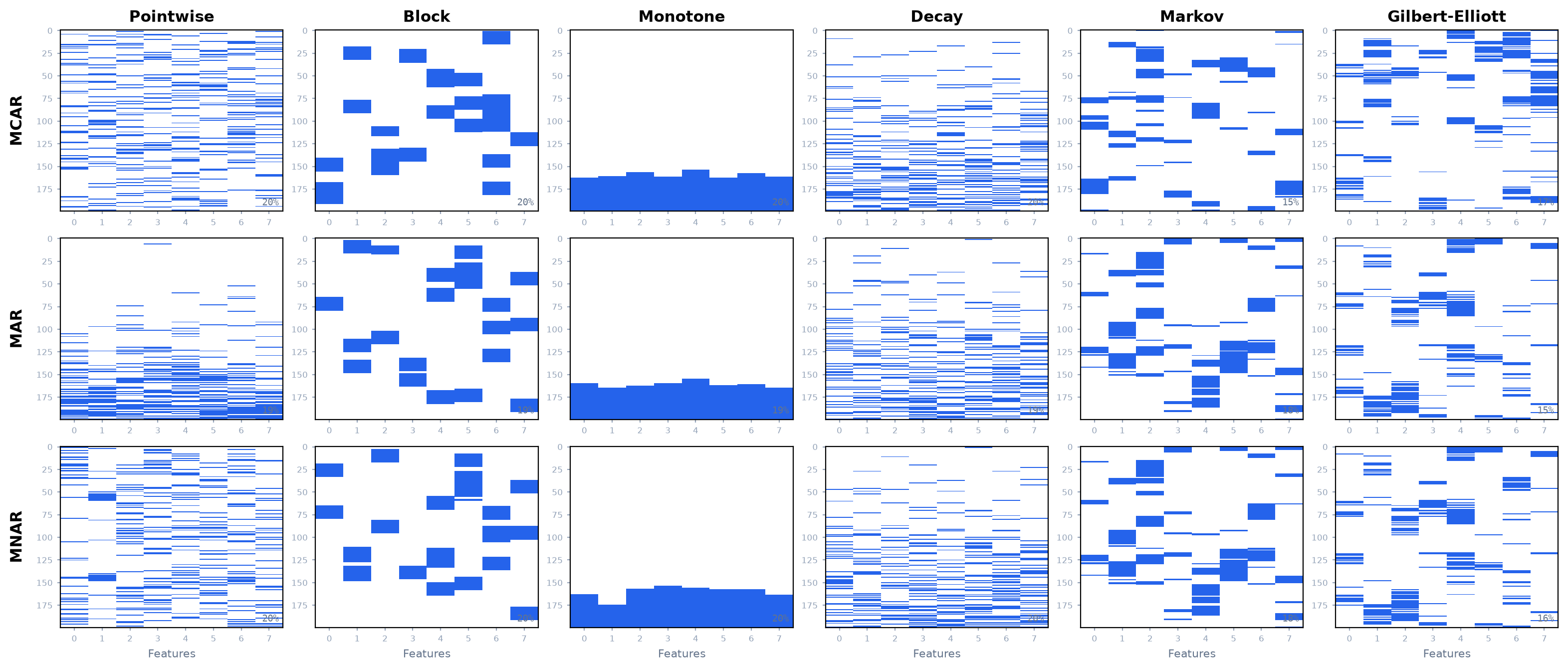
Pointwise

Individual values are missing as scattered points. This is the default.

X_missing, mask = simulate_missingness(X, "mcar", 0.15, seed=42)

Aliases: point, scattered.

Block

Missingness is arranged into contiguous segments, modeling sensor dropout or connectivity loss.

X_missing, mask = simulate_missingness(
    X, "mcar", 0.20, seed=42,
    pattern="block", block_len=10
)

By default, the block pattern uses a fixed block_len=10 and block_density=1.0, so all requested missingness is allocated to blocks. For long wearable-style time series, prefer block_frac to define block length relative to the time axis:

X_missing, mask = simulate_missingness(
    X, "mcar", 0.20, seed=42,
    pattern="block", block_frac=0.01
)

For a series with 30,000 timesteps, block_frac=0.01 creates blocks of about 300 timesteps. If both block_len and block_frac are provided, block_frac takes precedence.

To simulate variable-length dropout episodes, pass a (min_frac, max_frac) range. A new block length is sampled uniformly from the range for each block:

X_missing, mask = simulate_missingness(
    X, "mcar", 0.20, seed=42,
    pattern="block", block_frac=(0.01, 0.05)
)

Parameters:

Parameter	Default	Description
block_len	10	Length of each block in timesteps
block_frac	None	Relative block length as a fraction of the time axis, or (min_frac, max_frac) for variable-length blocks. Recommended for long time series.
block_density	1.0	Fraction of missingness allocated to blocks. Set below 1.0 to retain some pointwise missingness.

Alias: contiguous.

Monotone

Once a feature series becomes missing, all later eligible timesteps remain missing. This models participant dropout, study withdrawal, or permanent sensor failure.

X_missing, mask = simulate_missingness(
    X, "mcar", 0.20, seed=42, pattern="monotone"
)

Alias: dropout.

Temporal Decay

Missingness is shifted toward later timesteps using a sigmoid time ramp. This models gradual degradation, battery drain, or participant fatigue.

X_missing, mask = simulate_missingness(
    X, "mcar", 0.25, seed=42,
    pattern="decay", decay_rate=5.0, decay_center=0.6
)

Parameters:

Parameter	Default	Description
decay_rate	3.0	Steepness of the temporal ramp
decay_center	0.7	Normalized time of the 50% crossover

Alias: degradation.

Markov

Missingness follows a two-state Markov chain for each sample-feature series. The persist parameter controls how likely missingness is to continue once it starts.

X_missing, mask = simulate_missingness(
    X, "mcar", 0.20, seed=42,
    pattern="markov", persist=0.8
)

Parameters:

Parameter	Default	Description
persist	0.8	Probability of staying missing, in [0, 1)

Rate control: calibrated in expectation. The realized missing rate is approximate because each series is sampled from a Markov chain.

Alias: flickering.

Gilbert-Elliott

A two-state burst-loss model widely used to describe bursty packet loss in telecommunications. Each sample-feature series alternates between a good state (low loss) and a bad state (high loss). Unlike the markov pattern—where the bad state is always missing and the good state is never missing—Gilbert-Elliott produces ragged bursts: bad periods still let some values through, and good periods can have occasional dropouts.

X_missing, mask = simulate_missingness(
    X, "mcar", 0.20, seed=42,
    pattern="gilbert_elliott", persist=0.9,
    bad_loss=0.8, good_loss=0.02
)

Gilbert-Elliott currently supports only mechanism="mcar". Use markov if you need a bursty pattern that composes with MAR or MNAR.

For partial missing rates, calibration requires good_loss <= missing_rate < bad_loss; TSGap raises ValueError when the requested rate is outside that feasible range. With the defaults bad_loss=1.0 and good_loss=0.0, the model reduces to the clean on/off behavior of the markov pattern.

Gilbert-Elliott uses the MCAR mechanism mask to define the missingness budget over eligible entries, then reshapes that budget into a channel-style burst process. It preserves eligibility and target dimensions, but the final missing locations are governed by the hidden good/bad state process.

Parameters:

Parameter	Default	Description
persist	0.8	Probability of staying in the bad state, in [0, 1). Higher values create longer bursts.
bad_loss	1.0	Probability a value is missing while in the bad state (h), in (0, 1].
good_loss	0.0	Probability a value is missing while in the good state (k), in [0, 1). Must be strictly less than bad_loss.

Aliases: gilbert-elliott, gilbert, burst.

Gilbert-Elliott Edge Cases

• good_loss must satisfy 0 <= good_loss < bad_loss.

• bad_loss must satisfy 0 < bad_loss <= 1.

• persist must satisfy 0 <= persist < 1.

• For partial rates, good_loss <= missing_rate < bad_loss is required.

• If missing_rate=0, no new values are artificially masked.

• If missing_rate=1, all eligible values are masked, regardless of bad_loss and good_loss.

• With bad_loss=1.0 and good_loss=0.0, Gilbert-Elliott behaves like a clean on/off burst process similar to the markov pattern.

• With bad_loss<1.0, bad periods are leaky: some values remain observed inside bursts.

• With good_loss>0.0, good periods can still contain occasional isolated missing values.

Rate Control Summary

Different patterns control the target rate differently:

Pattern	Rate behavior
pointwise with MCAR	Exact count up to rounding
pointwise with MAR/MNAR	Calibrated probability, approximate realized rate
block	Preserves the mechanism missing count when enough eligible positions are available
monotone	Allocates the mechanism missing budget into dropout tails, with rounding adjustment
decay	Resamples the mechanism missing count using temporal weights
markov	Calibrated in expectation; realized rate is approximate
gilbert_elliott	MCAR-only. Calibrated in expectation when feasible; realized rate is approximate

Eligibility Guarantees

All patterns preserve:

• pre-existing NaNs as missing

• non-target dimensions as observed

• shape of the input data

• consistency between X_missing and mask